Overview
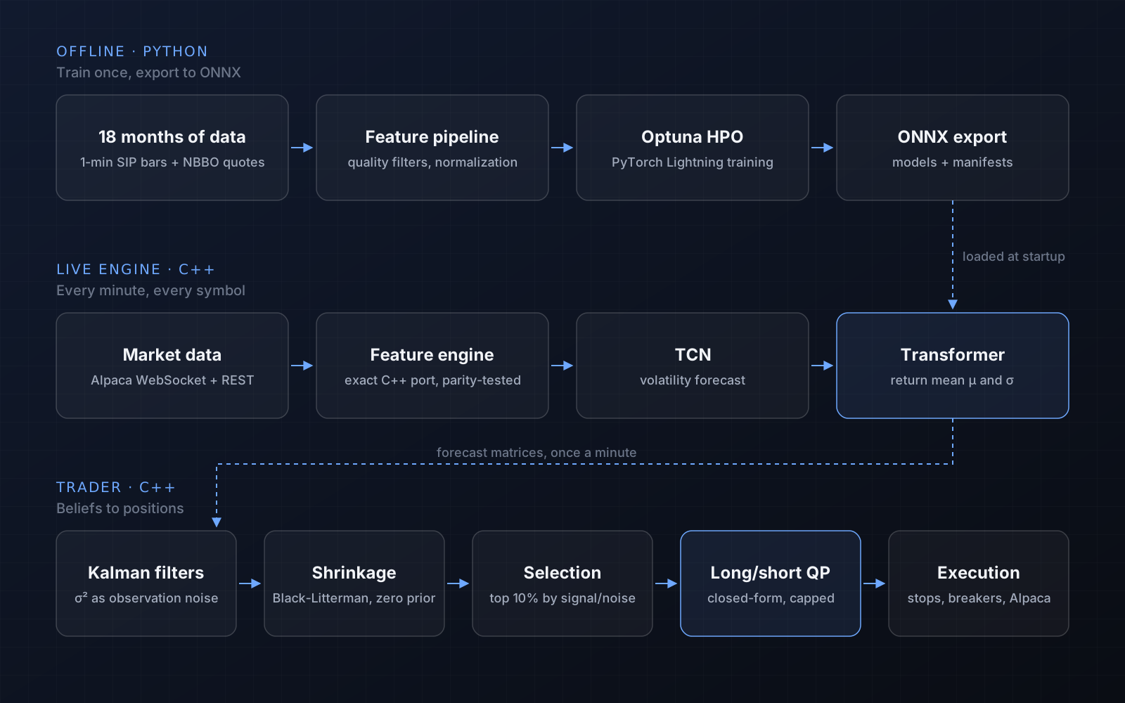
This started as a question: can a neural network trained on minute-level market data find signal a disciplined system can actually trade? Answering it honestly meant building much more than a model. It needed a data pipeline, a training and tuning setup, a real-time engine that reproduces the training features exactly, a portfolio layer that knows how confident each forecast is, and the risk controls that keep a live account safe.
Data
Training data is 18 months of 1-minute bars from the consolidated SIP feed for roughly 325 large-cap stocks, plus Level 1 quotes aggregated into a per-minute quoted spread. That's on the order of 45 million bars.
Market data has holes, and a model trained on holes learns nonsense, so the fetcher is strict:
- A session is dropped if it's missing more than 30 minutes or has a gap of 4 or more consecutive minutes.
- A whole symbol is dropped if more than 100 of its sessions fail that check.
- Early-close half days are skipped using the exchange calendar.
Normalization statistics are fit on the training split only and applied everywhere else, so no information leaks from validation or test data into training. Each example is a lookback window ending at time t; the target is the cumulative log return over the next 60 minutes. The lookback length is a tuned hyperparameter between 90 and 180 minutes.
Models
Two models, chained
A temporal convolutional network (TCN) forecasts each stock's realized volatility. That forecast becomes an input channel for the returns model, so the returns model always knows how turbulent the market expects the next hour to be.
Forecasting uncertainty, not just a number
The returns model doesn't output a single guess. It outputs a Gaussian distribution: a mean μ and a log-variance, trained with a heteroskedastic Gaussian negative log-likelihood with a beta-NLL weighting. In plain terms, the model learns to say how sure it is, minute by minute and stock by stock. That confidence turns out to be the most useful thing it produces.
Architectures I compared
Every model shares the same inputs and outputs, so they're interchangeable with one setting. I built and tuned an LSTM, a Transformer encoder, a modernized patch-based Transformer, and a mixture-of-experts that soft-routes five LSTMs through a learned gating network. Each model also learns an embedding per market sector. Hyperparameters were tuned with Optuna (TPE sampling, median pruning, parallel workers). The live system currently runs the Transformer.
The live engine
The live side is two C++20 programs. The inference engine ingests minute bars and quotes over a WebSocket, rebuilds the exact training features bar by bar, and runs both models through ONNX Runtime. The trader reads the forecasts and manages the portfolio.
- Feature parity. The C++ feature code is a line-for-line port of the Python pipeline, checked by tests against reference outputs from Python. If live features drift from training features, the model is silently wrong.
- Deterministic restarts. Start late, or crash mid-day, and the engine backfills every missed minute over REST and replays it through the same live code path. The forecasts after a 10:19 start are identical to a 9:30 start.
- Strict manifests. Each exported model carries a manifest with its lookback, feature list, and normalization. The engine refuses to start on any mismatch.
From forecasts to positions
A forecast isn't a trade. The trader turns forecasts into a portfolio in four layers, each feeding the next:
| Layer | What it does | Why |
|---|---|---|
| 1 · Kalman filters | Smooth each stock's forecast stream, using the model's own variance as the measurement noise | A minute the model marks uncertain barely moves the belief |
| 2 · Shrinkage | Black-Litterman update toward a prior of zero (no position) | Uncertain or stale beliefs fade out of the book on their own |
| 3 · Selection | Rank by expected move ÷ expected volatility; trade the top 10% | Only the clearest signals, long or short |
| 4 · Sizing | Mean-variance QP with leverage, position, and concentration caps | Solved exactly in closed form in microseconds |
The QP has a neat trick. Under a diagonal risk model, the best position never bets against its own forecast. So I fix each position's sign to the sign of its forecast, and the long/short problem becomes a long-only problem with a known closed-form solution. A unit test checks the two agree to 10⁻⁹.
Risk and execution
- Volatility-scaled trailing stops, with a cooldown before a stopped-out stock can be picked again.
- Drawdown circuit breakers that raise risk aversion and cut leverage in tiers.
- Limit orders near the mid, capped at 5% of recent volume, closing a third of each gap per cycle rather than lurching.
- A staged end-of-day unwind: stop adding, then unwind, then liquidate, then confirm flat.
- State saved to disk, so a restart keeps its stop levels and drawdown memory.
Code
Layer 1 in full. The key line is the measurement update: the Kalman gain k shrinks when the model's reported variance r is large, so uncertain forecasts move the belief less.
// Advance one time step with an EXPLICIT observation noise for this
// observation (the heteroskedastic model's own sigma_t^2). Pass NaN as y
// when the stream produced nothing this minute (time update only).
void step(double y, double r_obs) {
    const bool have_obs = std::isfinite(y);
    const double r = (std::isfinite(r_obs) && r_obs > 0.0) ? r_obs : r_;
    if (!initialized()) {
        if (have_obs) { m_ = y; p_ = r; }
        return;
    }
    p_ += q_;                                // time update
    if (have_obs) {                          // measurement update
        const double k = p_ / (p_ + r);
        m_ += k * (y - m_);
        p_ *= (1.0 - k);
    }
}
Live results
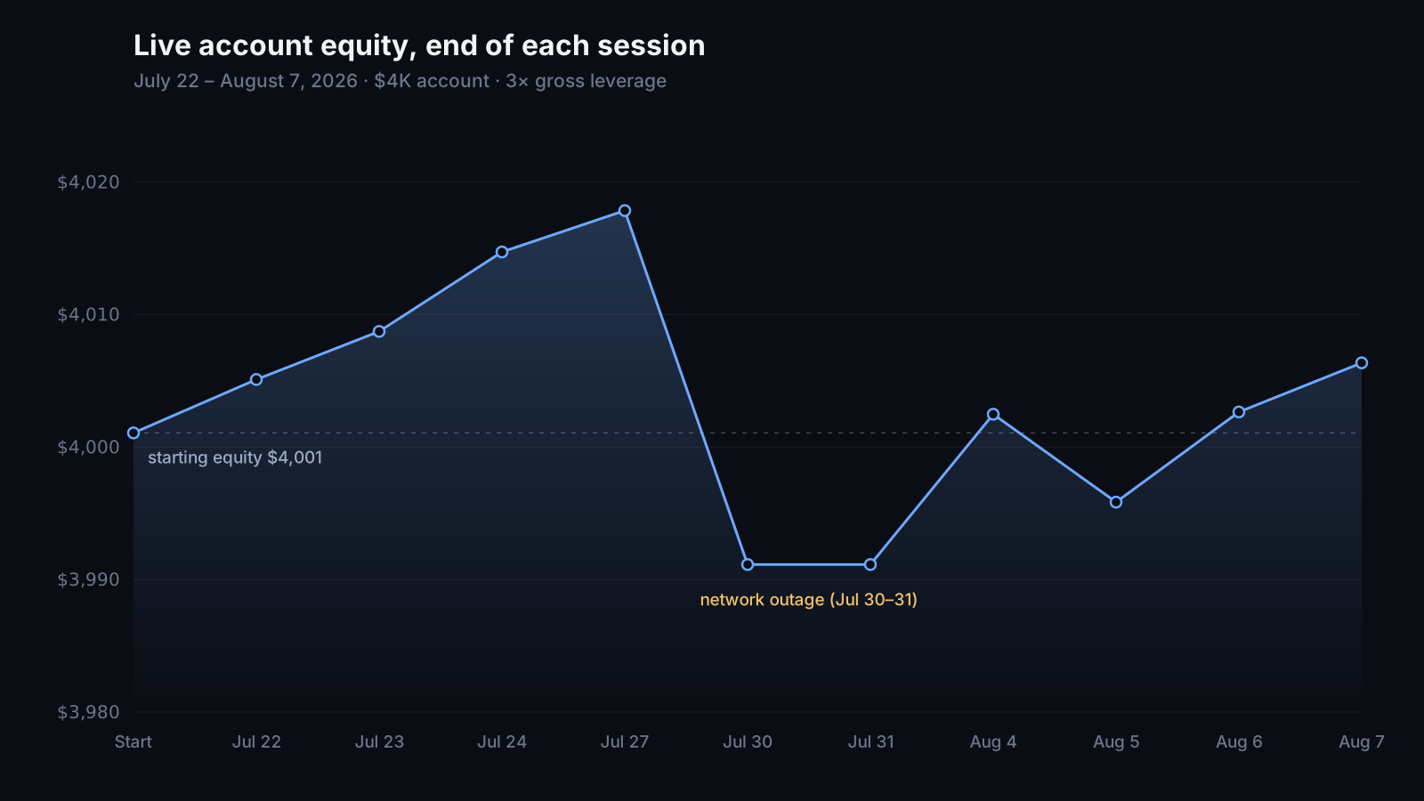
I ran the system live on a $4,000 account at 3× gross leverage for ten sessions in July and August 2026. These are the real numbers.
| Session | P&L | Notes |
|---|---|---|
| Jul 22 | +$4.02 | |
| Jul 23 | +$3.63 | |
| Jul 24 | +$6.00 | |
| Jul 27 | +$3.12 | |
| Jul 30 | −$26.71 | Network outage during the session |
| Jul 31 | $0.00 | Network outage during the session |
| Aug 4 | +$11.34 | |
| Aug 5 | −$6.63 | |
| Aug 6 | +$6.80 | |
| Aug 7 | +$3.71 | |
| Total | +$5.28 | 7 up, 2 down, 1 flat · +0.13% |
Seven of ten days were positive, but the net result is roughly break-even, and ten sessions is far too few to call anything. The honest conclusion is that the machinery works end to end in a live market. Whether the edge is real is a question for a proper walk-forward backtest, which is next.
The worst day came during a network outage. The trader couldn't reach the broker to check stops, and it logged a $0 closing balance because it couldn't read the account. No money was lost to that bug, but it showed me the trader needs to flatten or pause when it loses contact.
Version history
This is the third version. The first was a day-trading system built on a Temporal Fusion Transformer, trained on two years of minute data across the S&P 500. It used optimal-stopping theory (backward induction on a variant of the secretary problem) to decide when to enter, ATR-based trailing stops, and MILP position sizing, and it traded through the Schwab API. It ran for 19 days and averaged about 0.1% per day.
Its trailing stops meant positions were held only minutes, and pattern-day-trading rules limited how often it could trade. Those limits pushed the redesign toward what v3 is now: probabilistic forecasts, a portfolio that holds many long and short positions at once, and risk management built around the model's own uncertainty.
What I learned
- The model is maybe a fifth of the work. Data quality, feature parity, restart safety, and risk controls are the rest.
- Teaching a model to report its own uncertainty was worth more than squeezing extra accuracy out of its point forecast.
- Live trading finds failure modes backtests never will, like a flaky home network.
- Report results honestly, especially small or inconclusive ones.
Next: a walk-forward backtest to calibrate every strategy constant, a safe pause when the broker is unreachable, and a longer live run.